import pandas as pd
import numpy as np
import matplotlib as plt
import math
from IPython.display import Image

Agard model B

This validation case considers the AGARD-B model originally designed as a supersonic and later as a transonic wind tunnel calibration standard. The configuration is of interest as it is representative of wings and bodies used in slender body configurations where low aspect ratio wings of order 0·5 to 4 with swept back leading edges (> 45°) are commonly employed. The configuration consists of a sharp-nosed circular body with planar 60°-swept triangular delta wings of 4% thickness with a biconvex profile.

Experimental and numerical results are presented in the studies of Lombardi and Morelli (1995) Analysis of some interference effects in a transonic wind tunnel as well as Tuling et al. (2015) Compressible effects for the Agard-B model.

Initial conditions

The test case is non-dimensionalised so that an acoustic velocity of 1 is recovered for a temperature of 1. The non-dimensional material properties are

mP = pd.read_csv('./input/matProp.csv')
mP

	Gas constant	Specific heat ratio
0	287.058	1.4

and the freestream inlet conditions are

iCI = pd.read_csv('./input/intialCond.csv')
iCI

	Total pressure	Total temperature	Mach number
0	60000	315	0.8

From these the static values can be calculated using the isentropic flow equations. The static temperature is

mc=1.0+(mP.iloc[0][1]-1)/2*iCI.iloc[0][2]*iCI.iloc[0][2]
tempKelvin = iCI.iloc[0][1]*math.pow(mc,-1)
print("%.3f Kelvin" % tempKelvin)

279.255 Kelvin

and the static pressure reads

gc=-mP.iloc[0][1]/(mP.iloc[0][1]-1.)
staticPress= iCI.iloc[0][0]*math.pow(mc,gc)
print("%.3f N/m^2." % staticPress)

39361.297 N/m^2.

Experimental data is provided for an angle-of-attack ranging from -5 to 20$^\circ$, while numerically predicted normal force and pitching moments are determined for positive angles only due to symmetry.

Grid

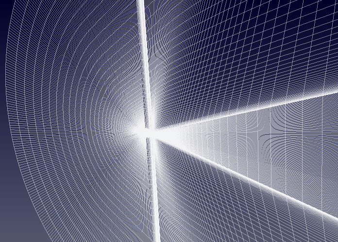
For the purpose of the analysis, a structured, half body mesh with 2·98million cells is created using the ICEM meshing software. At least 20 cells are used to resolve the boundary layer and for the first cell height a $y^+$ of approximately 1 is specified. The far-field boundaries are placed at least 20 body lengths away from the model. The surface mesh is shown below:

from IPython.display import Image, HTML, display
from glob import glob
imagesList=''.join( ["<img style='width: 600px; margin: 10px; float: left; border: 0px solid black;' src='%s' />" % str(s) 
                 for s in sorted(glob('screenShot/mesh/mesh*.png')) ])
display(HTML(imagesList))

Turbulence model

For the analysis the "Standard"-Spalart-Allmaras implementation is prescibed. Using Sutherland's Law $$\mu = \mu_{0} \left( \frac{T}{T_{0}} \right)^{3/2}\frac{T_{0} + S}{T + S}$$ and noting the requirements on the boundary conditions $$\tilde \nu_{wall} = 0, \quad 3 \nu_{\infty} < \tilde \nu_{\infty} < 5 \nu_{\infty}$$ the freestream value for $\tilde \nu_{\infty}$ can be calculated

# Sutherland
mu0 = 1.716e-5
T0  = 273.15
S   = 110.4
C1  = 1.458e-6
mu  = mu0*np.power(tempKelvin/T0,1.5)*(T0 + S)/(tempKelvin + S)
# Ideal gas density
rho = staticPress/(mP.iloc[0][0]*tempKelvin)
# print(rho)
# Kinematic viscosity
nu  = mu/rho
# Freestream nuTilda
nuTilda = 4*nu
print("%.4e m^2/s" % nuTilda)

1.4224e-04 m^2/s

To non-dimensionalise the integrated aerodynamic forces the following relations are employed to compute the body normal force $$ c_n = \frac{F_N}{\frac{1}{2} \rho u_i u_i A}$$ and pitching moment $$ c_{m} = \frac{M_m}{\frac{1}{2} \rho u_i u_i A c}$$ where $A$ and $c$ are the reference area and the centre of rotation respectively:

rV = pd.read_csv('./input/refValues.csv')
rV

	Length	Area	Centre of rotation
0	0.34641	0.155846	0.89145

Running

A number of scripts are provided to set up the case and run the simulation. To convert the ICEM mesh to the FOAM format, navigate to the case directory, agardB, and execute the scripts ./cleanMesh and ./setupMesh. The setupMesh script executes the following commands:

fluent3DMeshToFoam	Converts the ICEM mesh to the FOAM format
createPatch	Renames the patch surfaces

Next, to set up and run a batch of simulations for different angles-of-attack the following input files and scripts are provided:

runs	Matrix with input conditions
settings	Other, constant, input conditions
~removeDirs	Delete the simulation directories listed in the test matrix
setupDirs	Setup the simulation directories listed in the test matrix
submitRuns	Run the simulations

Results

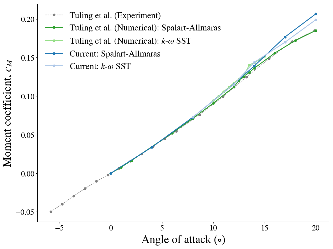
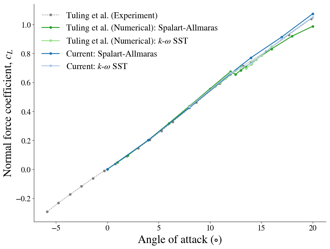
To evaluate the numerical prediction, the pitching moment coefficient and normal force are compared to the experimental and numerical data presented by Tuling et al. (2015).

from IPython.display import Image, HTML, display
from glob import glob
imagesList=''.join( ["<img style='width: 650px; margin: 5px; float: left; border: 0px solid black;' src='%s' />" % str(s) 
                 for s in sorted(glob('screenShot/results/aoa*.png')) ])
display(HTML(imagesList))

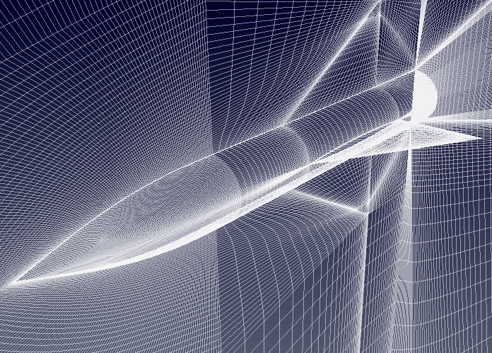
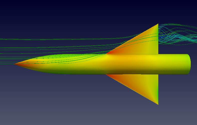
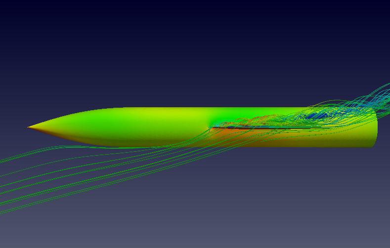
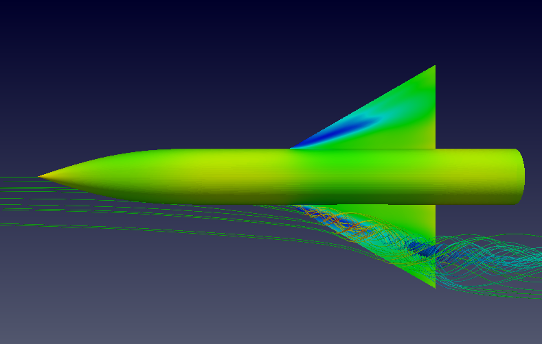
Below, the streamlines with vortex formation for an angle-of-attack of 16$^\circ$ are shown.

from IPython.display import Image, HTML, display
from glob import glob
imagesList=''.join( ["<img style='width: 650px; margin: 5px; float: left; border: 0px solid black;' src='%s' />" % str(s) 
                 for s in sorted(glob('screenShot/results/agard*.png')) ])
display(HTML(imagesList))

from IPython.core.display import HTML

def css_styling():
    styles = open("./styles/custom.css", "r").read()
    return HTML(styles)
css_styling()