import pandas as pd
import numpy as np
import matplotlib as plt
import math
from IPython.display import Image, HTML, display
from glob import glob
Basic finner
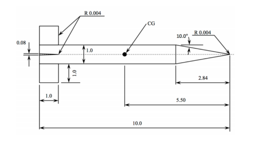
The basic finner or Army-Navy generic finner missile (ANF) considers a generic missile configuration for which longitudinal stability coefficients are available for Mach numbers in a range of 0.5-4.5
References
- Allen et al. (2017) Forced motions design for aerodynamic identification and modelling of a generic missile configuration.
- Bhagwandin and Sahu (2013) Numerical prediction of pitch damping stability derivatives for finned projectiles.
Below, a schematic representation of the generic configuration is shown:
imagesList=''.join( ["<img style='width: 410px; margin: 10px; float: left; border: 0px solid black;' src='%s' />" % str(s)
                 for s in sorted(glob('screenShot/geo/anfSchem.png')) ])
display(HTML(imagesList))
Initial conditions
Assuming the ideal gas approximation, the material properties are
mP = pd.read_csv('./input/matProp.csv')
mP
and the specified freestream inlet conditions are
iCI = pd.read_csv('./input/intialCond.csv')
iCI
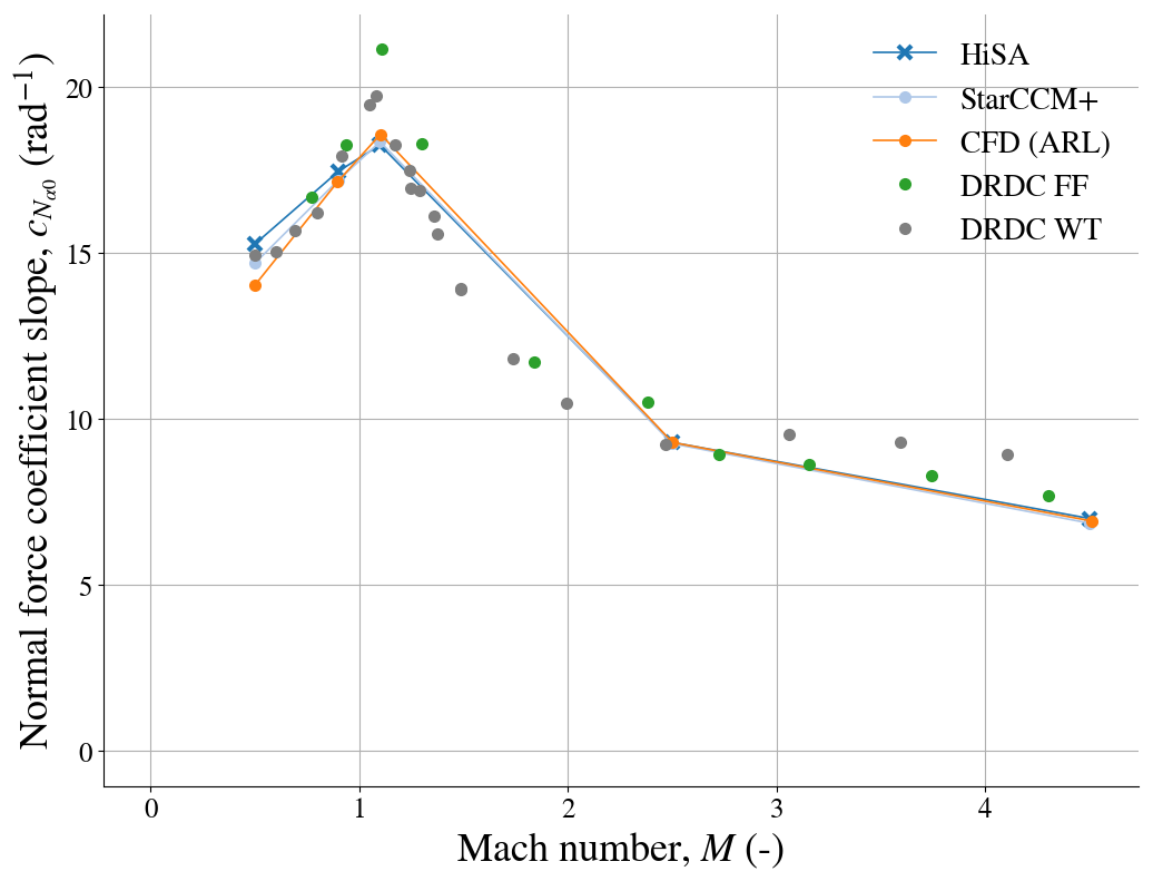
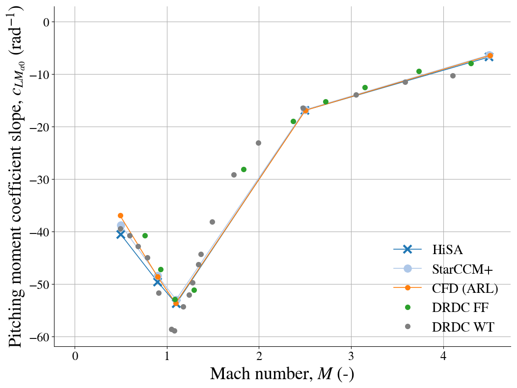
Experimental results for the static aerodynamic coefficients, namely, the axial force, the normal force slope and pitching moment slope at 0$^\circ$, are available.
Grid
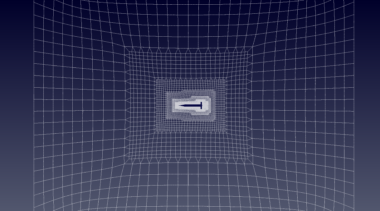
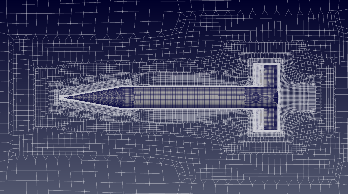
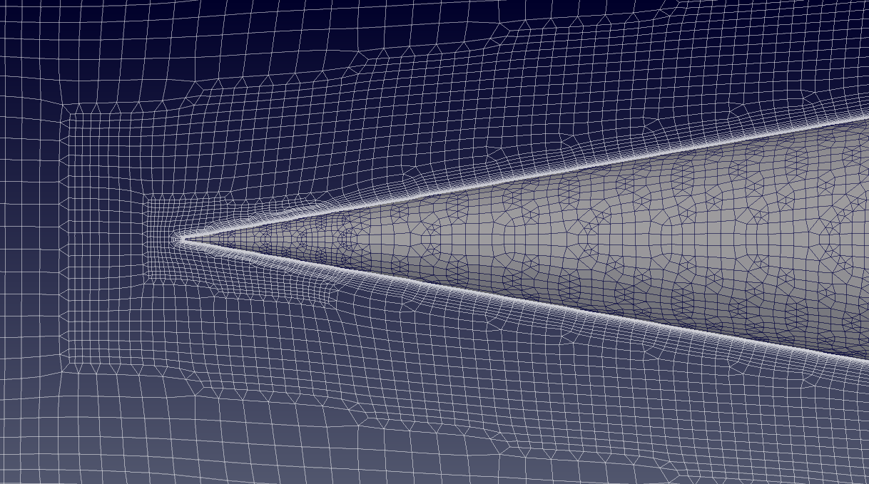
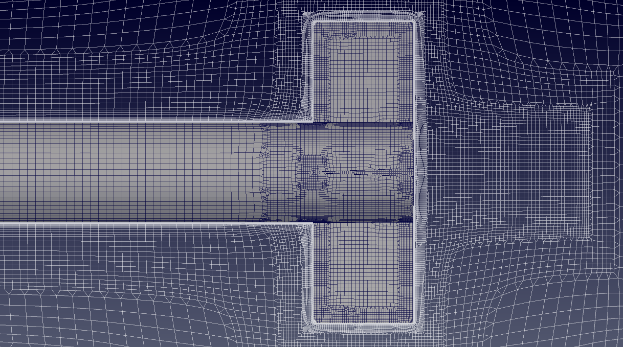
For the purpose of the analysis, an unstructured, cut-cell Cartesian mesh with approximately 2 million cells is created using the hexPress utility. The viscous sublayer is resolved and an expansion ratio of 1.2 is used in the boundary layer. To resolve the sublayer a non-dimensional first cell height or $y^+$ of less than 1 is required. The farfield boundaries are placed 50 characteristic lengths away. The surface mesh is shown below
imagesList=''.join( ["<img style='width: 650px; margin: 10px; float: left; border: 0px solid black;' src='%s' />" % str(s)
                 for s in sorted(glob('screenShot/mesh/mesh*.png')) ])
display(HTML(imagesList))
Turbulence model
For the analysis the "Standard"-Menter SST implementation is prescibed. If a turbulent intensity, $I$, of 1% and mixinglength, $L$, of 1x10$^{-5}$ m are prescibed, the corresponding farfield $k$ and $\omega$ values can be calculated from the relations $$ k = \frac{3}{2} (I |U|)^2$$ $$ \omega = \frac{\sqrt{k}}{C_{\mu}^{0.25} L}$$ where $C_{\mu} = 0.09$
# Ideal gas density
# rho = iCI.iloc[0][0]/(mP.iloc[0][0]*iCI.iloc[0][1])
c = math.sqrt(mP.iloc[0][1]*mP.iloc[0][0]*iCI.iloc[0][1])
for index, row in iCI.iterrows():
    M = iCI.iloc[index][2]
    u = M*c
    k = 3/2*(0.01*u)**2
    omega = math.sqrt(k)/(math.pow(0.9,0.25)*1e-5)
    print("For Mach = {} -> k = {:.1f} and omega = {:.1f}".format(M,k,omega))
For the non-slip wall the following wall functions are selected: kqRWallFunction, omegaWallFunction, nutkWallFunction and alphatWallFunction
To non-dimensionalise the integrated aerodynamic forces the following relations are employed to compute the body normal force $$ c_n = \frac{F_N}{\frac{1}{2} \rho u_i u_i A}$$ and pitching moment $$ c_{m} = \frac{M_m}{\frac{1}{2} \rho u_i u_i A c}$$ where $A$ and $c$ are the reference area and the centre of rotation respectively.
rV = pd.read_csv('./input/refValues.csv')
rV
The freestream viscosity is computed using Sutherland's Law $$\mu = \mu_{0} \left( \frac{T}{T_{0}} \right)^{3/2}\frac{T_{0} + S}{T + S}$$
# Sutherland
mu0 = 1.716e-5
T0  = 273.15
S   = 110.4
C1  = 1.458e-6
mu  = mu0*np.power(iCI.iloc[0][1]/T0,1.5)*(T0 + S)/(iCI.iloc[0][1] + S)
# Ideal gas density
rho = iCI.iloc[0][0]/(mP.iloc[0][0]*iCI.iloc[0][1])
# print(rho)
# Kinematic viscosity
nu  = mu/rho
The corresponding Reynolds number is computed using the relation $$\mathrm{Re} = \frac{\rho u L}{\mu}$$ from which the first cell height can be computed using the $y^+$ approximation. When wall functions are employed, a $y^+$ between 30 and 150 is required.
c = math.sqrt(mP.iloc[0][1]*mP.iloc[0][0]*iCI.iloc[0][1])
for index, row in iCI.iterrows():
    M = iCI.iloc[index][2]
    u = M*c
#     Re = rho*u*rV.iloc[0][0]/mu
    len = 0.3
    Re = rho*u*len/mu
    if (Re > 1e9):
        print ("******************************************************************************")
        print ("WARNING: The Schlichting skin-friction correlation is only valid for Re < 10e9")
        print ("******************************************************************************")
    # Schlichting skin-friction correlation
    Cf    = np.power(2*np.log10(Re)-0.65,-2.3)
    # Wall shear stress
    tauW  = 0.5*Cf*rho*u*u
    # Friction velocity
    uStar = np.sqrt(tauW/rho)
    # Wall distance
    yPlus = 1
    y     = yPlus*mu/(rho*uStar)
    print("For Mach = {} -> Re = {:.1e} and y(y+={}) = {:.1e} m".format(M,Re,yPlus,y))
Results
Below, the normal force and pitching moment slopes are compared to numerical results from the Army Research Lab as well as experimental data from Defence Research and Development Canada (DRDC). The slopes for both static wind tunnel tests (WT) and free flight (FF) are available.
from IPython.display import Image, HTML, display
from glob import glob
imagesList=''.join( ["<img style='width: 650px; margin: 5px; float: left; border: 0px solid black;' src='%s' />" % str(s)
                 for s in sorted(glob('screenShot/results/aero*.png')) ])
display(HTML(imagesList))
from IPython.core.display import HTML

def css_styling():
    styles = open("./styles/custom.css", "r").read()
    return HTML(styles)
css_styling()