import pandas as pd
import numpy as np
import matplotlib as plt
from IPython.display import Image

Mach 3.0 wind tunnel with a step

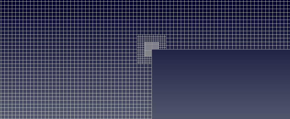
This validation case consideres the Mach 3.0 wind tunnel with a step as presented in the study of Woodward and Colella (1984) The numerical simulation of two-dimensional fluid flow with strong shocks. A rarefraction fan forms at the corner of the step resulting a singularity. With most numerical formulations this singularity introduces an erroneous entropy layer along the wall of the step and subsequently a spurious Mach stem at the bottom wall. For this analysis no special numerical treatment is applied; instead, an additional two levels of mesh refinement are applied at the step corner to reduce these numerical artifacts.

Additional literature resources include:

• Cockburn and Shu (1998) The Runge–Kutta Discontinuous Galerkin Method for Conservation Laws
• Greenshields et al. (2009) Implementation of semi-discrete, non-staggered central schemes in a colocated, polyhedral, finite volume framework, for high-speed viscous flows

Initial conditions

The test case is non-dimensionalised so that an acoustic velocity of 1 is recovered for a temperature of 1. The non-dimensional material properties are

mP = pd.read_csv('./input/matProp.csv')
mP

	Gas constant	Specific heat ratio
0	0.714	1.4

and the specified, non-dimensional inlet conditions are

iCI = pd.read_csv('./input/intialCond.csv')
iCI

	Pressure	Temperature	Velocity
0	1.0	1.0	3.0

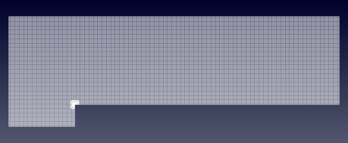
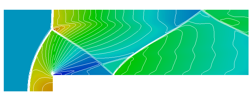
Grid

For the purpose of the analysis a two-dimensional structured mesh is generated using the blockMesh utility. For the fine mesh the cell size corresponds to a characteristic length of $\frac{1}{120}$. As noted previously, two additional levels of h-refinement are applied in the region of the step corner.

from IPython.display import Image, HTML, display
from glob import glob
imagesList=''.join( ["<img style='width: 600px; margin: 10px; float: left; border: 0px solid black;' src='%s' />" % str(s) 
                 for s in sorted(glob('screenShot/mesh/mesh*.png')) ])
display(HTML(imagesList))

Running

A script is provided to set up the case and run the simulation. The script ./runSim generates the mesh, applies additional refinement at the corner and runs the simulation.

Results

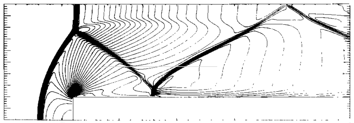
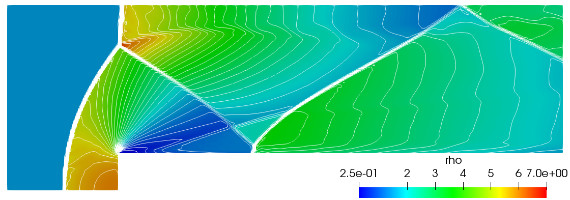
To validate the numerical prediction, the density contours for the AUSM$^{+}$up and Kurganov shock capturing schemes are compared with the results from Woodward and Colella (1984) at 4 seconds. Although the various methods show good correlation when comparing the principal flow features, both the Woodward and Colella scheme (top) and AUSM$^{+}$up (middle) show some numerical artifacts from the entropy layer at the Mach stem on the step wall while Kurganov and Tadmor's scheme does not seem to exibit this.

from IPython.display import Image, HTML, display
from glob import glob
imagesList=''.join( ["<img style='width: 510px; margin: 10px; float: left; border: 0px solid black;' src='%s' />" % str(s) 
                 for s in sorted(glob('screenShot/results/rho*.png')) ])
display(HTML(imagesList))

from IPython.core.display import HTML

def css_styling():
    styles = open("./styles/custom.css", "r").read()
    return HTML(styles)
css_styling()