import pandas as pd
import numpy as np
import matplotlib as plt
from IPython.display import Image
Agard 445.6
This validation case consideres the transonic flutter analysis of the weakend, Agard 445.6 model 3 as presented in Yates et al. (1963). For validation purposes, the study presents numerical results from the High Speed Aerodynamic solver (HiSA) using a modal structural method and compares it to published numerical results as well as experimental measurements.
Additional literature resources include:
- Chwalowski et al. (2011) Preliminary computational analysis of the HIRENASD configuration in preparation for the aeroelastic prediction workshop
- Pahlavanloo (2007) Dynamic Aeroelastic Simulation of the AGARD 445.6 Wing using Edge
- Lee-Rausch & Batina (1993b) Calculation of Agard 445.6 flutter using Navier-Stokes aerodynamics
Material properties
It is assumed the fluid can be treated as an ideal gas and uses the following material properties
mP = pd.read_csv('./input/matProp.csv')
mP
Initial conditions
The experimental study evaluated the flutter threshold and is summarised in the table below. To numerically determine the onset of flutter, the velocity and temperature are fixed for each control point and a pressure sweep is performed. Each simulation conducted during the pressure sweep consists of a steady analysis assuming a rigid or fixed structure to initialise the flow field followed by a transient simulation that allows for structural deformation. Since a symmetric airfoil is considered and the tests are performed at a zero angle of attack, a static aeroelastic analysis is not required.
iCI = pd.read_csv('./input/intialCond.csv')
iCI
Grid
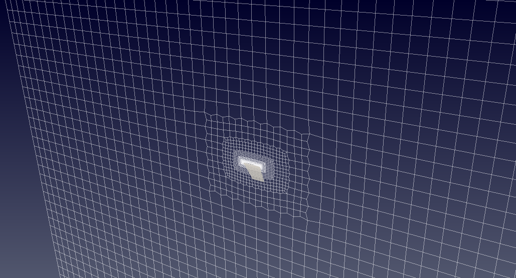
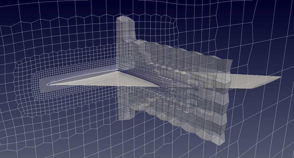
For the purpose of the analysis a cut-cell Cartesian mesh is generated using cfMesh. Note that in order to support the adaptive mesh refinement used in this example, the customised version of cfMesh available from https://gitlab.com/hisa/cfMesh, must be downloaded and compiled before running this case.
The model uses a symmetric NACA 65A004 profile. The wing is swept 45 degrees at the quater line chord, has a span of 0.762 m and a taper ratio of 0.66. For the purpose of this study, inviscid flow is assumed and the boundary layer is therefore not resolved.
from IPython.display import Image, HTML, display
from glob import glob
imagesList=''.join( ["<img style='width: 610px; margin: 10px; float: left; border: 0px solid black;' src='%s' />" % str(s)
                 for s in sorted(glob('screenShot/mesh/mesh*.png')) ])
display(HTML(imagesList))
Modal analysis
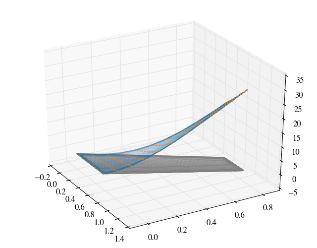
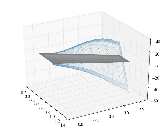
The modal data was taken from Yates (1987) which were normalised to a unit modal mass in lbf-in-s$^2$ or 175.1268 kg and the frequencies of the 1, 2 and 3 modes are respectively 9.5992, 38.1650 and 48.3482 Hz.
rV = pd.read_csv('./input/refValues.csv')
rV
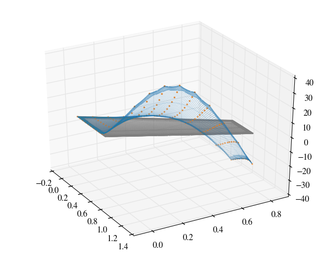
The modeshapes are interpolated on to the surface patch of the wing and are shown below.
from IPython.display import Image, HTML, display
from glob import glob
imagesList=''.join( ["<img style='width: 230px; margin: -10px; float: left; border: 0px solid black;' src='%s' />" % str(s)
                 for s in sorted(glob('screenShot/results/mode*.png')) ])
display(HTML(imagesList))
Running
A number of scripts are provided to set up the case and run the simulation. To generate the mesh, navigate to the case directory, agard445, and execute the scripts ./cleanMesh and ./setupMesh. The setupMesh script executes the following commands:
| surfaceFeatureEdges | Extract the feature edges for cfMesh |
| cartesianMesh | Creates a cut-cell Cartesian mesh using the cfMesh utility |
| createPatch | Renames the boundary patches and sets the patch types |
To generate the mode shapes and interpolate them onto the wing surface patch from the experimental data the genModeShape script is provided.
Next, to setup and run the batch of simulations for the Mach number and pressure sweeps the following bash and python scripts are provided.
| runs | Test matrix with input conditions |
| ~removeDirs | Delete the simulation directories listed in the test matrix |
| setupDirs | Setup the simulation directories listed in the test matrix |
| submitRuns | Submit and run the simulations on either a local workstation or network cluster |
| runSimFixed | Located in the simulation directory, this script runs the steady or static simulation to initialise the flow field. |
| runSimTransient | Located in the simulation directory, this script copies the initialised flow field and execute the transient analysis. |
Results
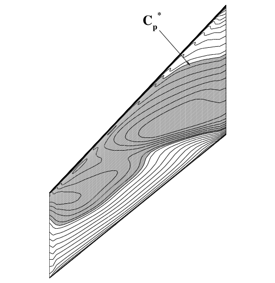
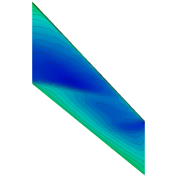
For an angle-of-attack of 0$^\circ$ and M=0.96, the pressure contour for the static, Euler analysis is shown below. The figure on the left is taken from Rausch and Batina (1993) and on the right the pressure computed using HiSA is plotted.
from IPython.display import Image, HTML, display
from glob import glob
imagesList=''.join( ["<img style='width: 310px; margin: 10px; float: left; border: 0px solid black;' src='%s' />" % str(s)
                 for s in sorted(glob('screenShot/results/press*.png')) ])
display(HTML(imagesList))
From the aeroelastic simulations the flutter boundary may be computed and compared to measurements as well as numerical results presented in literature. The flutter boundary or stability limit follows the zero aerodynamic damping line; at higher dynamic pressures the system becomes unstable.
In order to compare against other results, the Flutter Speed Index (FSI) is plotted. This is defined as
$\text{FSI} = \frac{U_f}{b_s\omega_{\alpha}\sqrt{\mu}}$
where
- $U_f$ is the flutter speed
- $b_s = 0.2794$ m is the root semi-chord
- $\omega_\alpha = 2\pi*38.10$ rad/s is the angular frequency of the first torsion mode
- $\mu$ is the mass ratio, $\mu = \frac{\hat{m}}{\rho_f V}$
- $\hat{m} = 1.862$ kg is the wing panel mass
- $\rho_f$ is the free-stream density at flutter
- $V$ is the volume of a truncated cone with top and bottom radii equal to the root and tip semi-chords, and height equal to the span, i.e. $V = \frac{\pi}{3}s(b_s^2+b_t^2+b_sb_t)$.
- $s = 0.762$ m is the span
- $b_t = 0.1841$ m is the tip semi-chord
Thus, FSI can be written as
$\text{FSI} = \frac{\sqrt{2p_d}}{{b_s\omega_\alpha\sqrt{\hat{m}/V}}}$
where $p_d = \frac12\rho_f U_f$ is the dynamic pressure at flutter.
The flutter speed index is plotted below against various other results.
from IPython.display import Image, HTML, display
from glob import glob
imagesList=''.join( ["<img style='width: 650px; margin: 10px; float: left; border: 0px solid black;' src='%s' />" % str(s)
                 for s in sorted(glob('screenShot/results/flutterSpeedIndex.svg')) ])
display(HTML(imagesList))

- The experimental result is from Yates et al. (1963)
- The first four computational results are as summarised by Goura (2001) and the other three as summarised by Pahlavanloo (2007). The original reference is given in the figure legend, where it is known.
References
- Yates et al. (1963) Measured flutter and calculated characteristics in air and in Freon-12 in the Langley transonic dynamics tunnel, NASA Technical Note D-1616. In Yates (1987) AGARD standard aeroelastic configurations for dynamic response, NASA Technical Memorandum 100492
- Yates (1987) AGARD standard aeroelastic configurations for dynamic response, NASA Technical Memorandum 100492
- Lee-Rausch & Batina (1993a) Wing flutter boundary prediction using an unsteady Euler aerodynamic method, NASA Technical Memorandum 107732
- Lee-Rausch & Batina (1993b) Calculation of AGARD 445.6 flutter using Navier-Stokes aerodynamics, AIAA Paper 93-3476
- Gupta (1996) Development of a Finite Element Aeroelastic Analysis Capability, Journal of Aircraft 33(5)
- Lesoinne & Farhat (1998) High order subiteration-free staggered algorithm for nonlinar transient aeroelastic problems, AIAA Journal 36(9) p. 1626
- Goura (2001) Time marching analysis of flutter using computational fluid dynamics, PhD Thesis, University of Glasgow
- Pahlavanloo (2007) Dynamic Aeroelastic Simulation of the AGARD 445.6 Wing using Edge, FOI Technical Report FOI-R--2259--SE
- Chwalowski et al. (2011) Preliminary computational analysis of the HIRENASD configuration in preparation for the aeroelastic prediction workshop, International Forum on Aeroelasticity and Structural Dynamics IFASD-2011-108
from IPython.core.display import HTML

def css_styling():
    styles = open("./styles/custom.css", "r").read()
    return HTML(styles)
css_styling()