import pandas as pd
import numpy as np
import matplotlib as plt
from IPython.display import Image
Mach 4.5 Turbulent Flow over a Flat Plate
This validation case consideres Mach 4.5 Turbulent Flow over a Flat Plate from the NPARC Alliance Validation and Verification Archive. Below, the results from the high speed aerodynamic solver (HiSA) are compared to the results from WIND.
Material properties
As the working fluid considered is air, the fluid can be treated as an ideal gas and the following material properties are assumed:
mP = pd.read_csv('./input/matProp.csv')
mP
Initial conditions
The NPARC archive provides the follow input parameters, in imperial units, for the freestream conditions:
iCI = pd.read_csv('./input/intialCondImp.csv')
iCI
From these the input parameters, SI units for HiSA are computed. The freestream or static temperature, $T$, in Kelvin is
tempKelvin = iCI.iloc[0][2]*5.0/9.0
print("%.3f K" % tempKelvin)
and the freestream presure, $p_{\infty}$, in Pascals is
pressPascal = iCI.iloc[0][1]*6894.75729
print("%.3f Pa" % pressPascal)
If the acoustic velocity, $c$, is
c = np.sqrt(mP.iloc[0][1]*mP.iloc[0][0]*tempKelvin)
print("%.3f m/s" % c)
then the prescribed inlet velocity, $u$, vector is
u = iCI.iloc[0][0]*c
ux = u*np.cos(iCI.iloc[0][3]*np.pi/180.0)
uy = u*np.sin(iCI.iloc[0][3]*np.pi/180.0)
print("( %.3f 0.0 %.3f ) m/s if AoA = %.2f" % (ux,uy,iCI.iloc[0][3]))
Grid
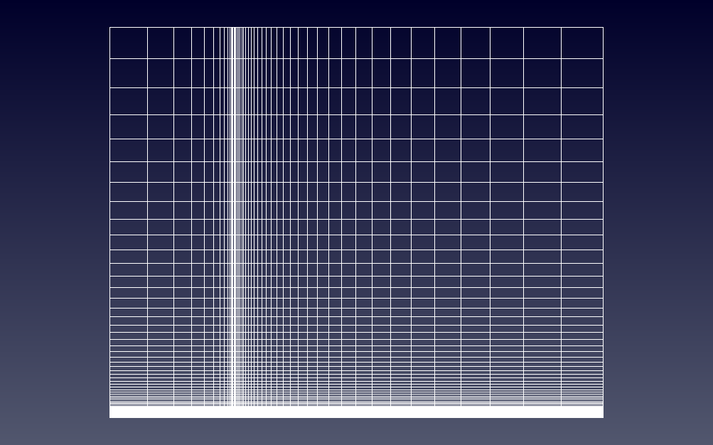
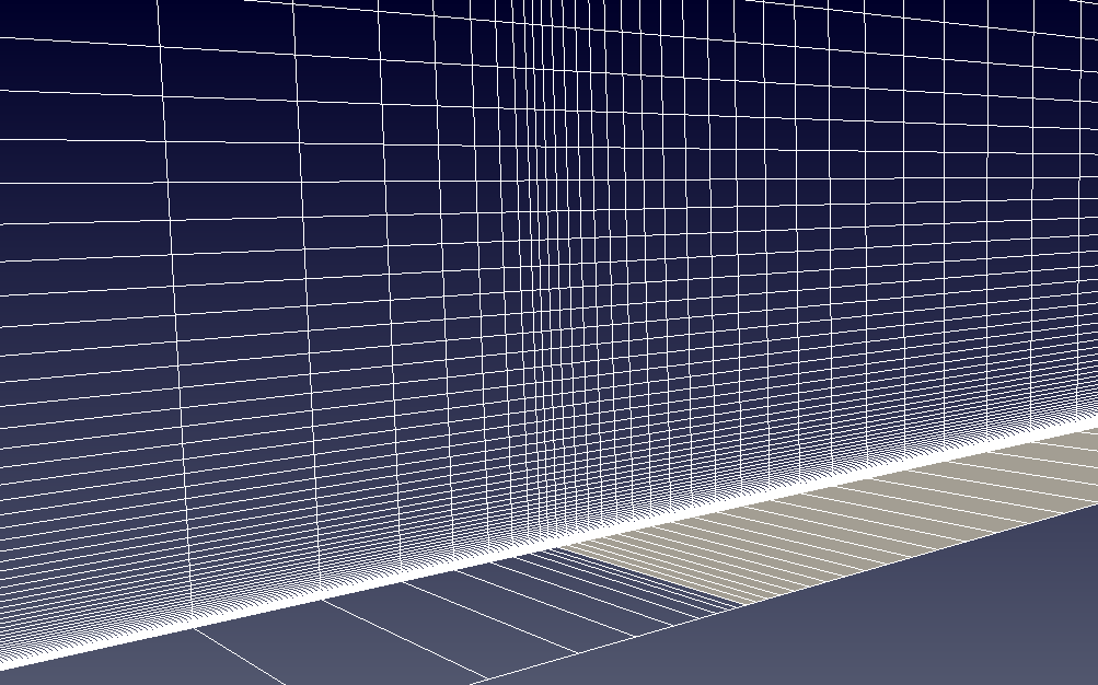
A two-dimensional, structured mesh is generated using the blockMesh utility. Similar to the structured mesh provided by NPARC, the grid consists of 60 points in the streamwise (x-) direction and 10 points in the transverse (y-) direction. In the streamwise direction, the grid is packed at x=0, the beginning of the viscous wall. To ensure that the boundary layer was resolved, the grid is packed in the transverse direction to a nominal spacing of $y^+$=1.0 along the lower boundary.
from IPython.display import Image, HTML, display
from glob import glob
imagesList=''.join( ["<img style='width: 500px; margin: 10px; float: left; border: 0px solid black;' src='%s' />" % str(s)
                 for s in sorted(glob('screenShot/mesh/mesh*.png')) ])
display(HTML(imagesList))
Turbulence model
For the analysis the "Standard"-Spalart-Allmaras implementation is prescibed. Using Sutherland's Law $$\mu = \mu_{0} \left( \frac{T}{T_{0}} \right)^{3/2}\frac{T_{0} + S}{T + S}$$ and noting the requirements on the boundary conditions $$\tilde \nu_{wall} = 0 \quad \text{and} \quad 3 \nu_{\infty} < \tilde \nu_{\infty} < 5 \nu_{\infty}$$ the freestream value for $\tilde \nu_{\infty}$ can be calculated:
# Sutherland
mu0 = 1.716e-5
T0  = 273.15
S   = 110.4
C1  = 1.458e-6
mu  = mu0*np.power(tempKelvin/T0,1.5)*(T0 + S)/(tempKelvin + S)
# Ideal gas density
rho = pressPascal/(mP.iloc[0][0]*tempKelvin)
# print(rho)
# Kinematic viscosity
nu  = mu/rho
# Freestream nuTilda
nuTilda = 4*nu
print("%.4e m^2/s" % nuTilda)
For the flat plate, the reference length is taken to be that of the plate.
rV = pd.read_csv('./input/refValues.csv')
rV
The corresponding Reynolds number, $\mathrm{Re}$, is
Re = rho*u*rV.iloc[0][0]/mu
print("%.2f" % Re)
To recover a $y^+$ of 1, the wall distance, $y$, should be less than
if (Re > 1e9):
    print ("******************************************************************************")
    print ("WARNING: The Schlichting skin-friction correlation is only valid for Re < 10e9")
    print ("******************************************************************************")
# Schlichting skin-friction correlation
Cf    = np.power(2*np.log10(Re)-0.65,-2.3)
# Wall shear stress
tauW  = 0.5*Cf*rho*u*u
# Friction velocity
uStar = np.sqrt(tauW/rho)
# Wall distance
yPlus = 1
y     = yPlus*mu/(rho*uStar)
print("%.4e m" % y)
and for $y^+$ of 30, $y$ should be smaller than
yPlus = 30
y     = yPlus*mu/(rho*uStar)
print("%.4e m" % y)
Running
A number of scripts are provided to set up the case and run the simulation. To generate the mesh, navigate to the case directory, flatPlate, and execute the scripts ./cleanMesh and ./setupMesh. The setupMesh script executes the following command:
| blockMesh | Generate a block structured mesh |
Next, to run the simulation the ./cleanSim and ./runSim scripts should be executed. The runSim script creates a symbolic link to the mesh files in the folder mesh and executes the solver across multiple cores.
Convergence
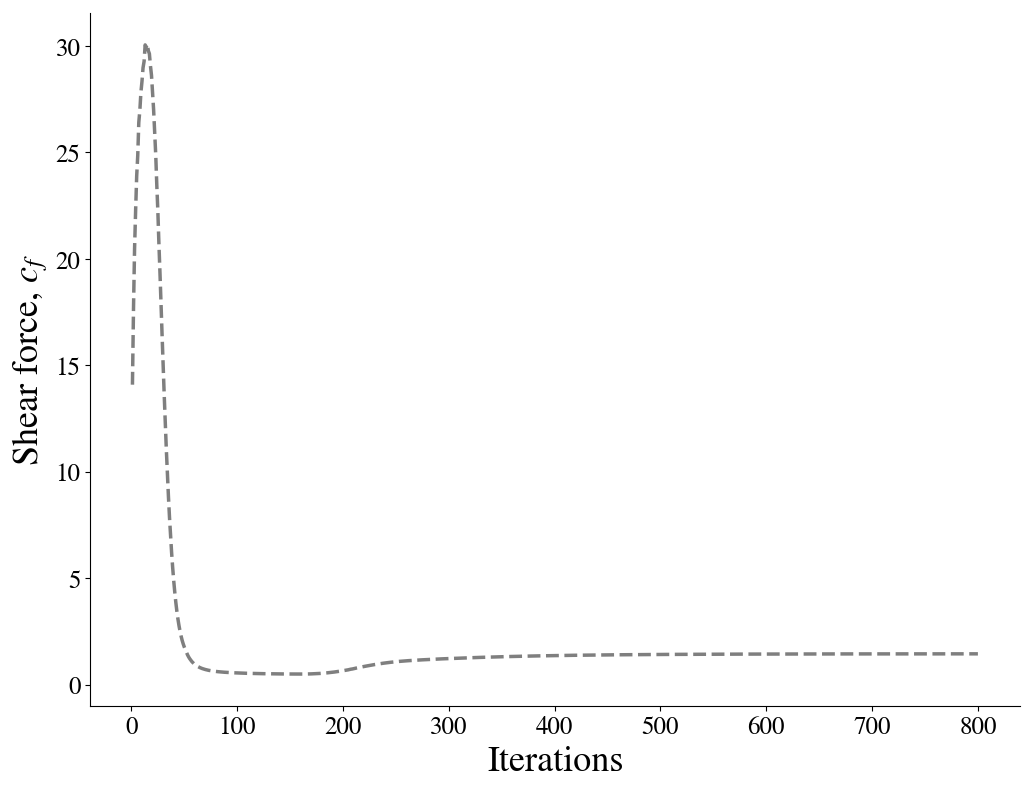
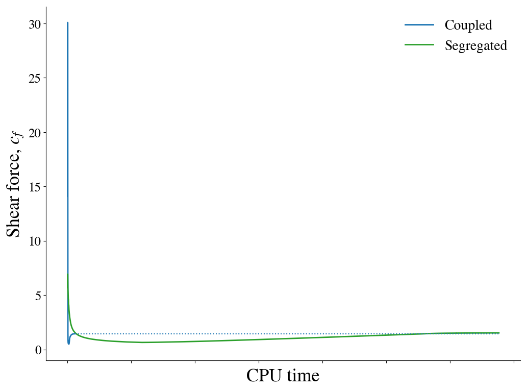
To examine the solution convergence, first the engineering quantities are evaluated. In the upper figure, the shear friction coefficient is plotted against the number of iterations. In the lower figure, the convergence as a function of CPU time is shown for both the coupled solver as well as a segregated approach, demonstrating the improvement in solution time.
from IPython.display import Image, HTML, display
from glob import glob
imagesList=''.join( ["<img style='width: 415px; margin: 10px; float: left; border: 0px solid black;' src='%s' />" % str(s)
                 for s in sorted(glob('screenShot/results/*Conv*.png')) ])
display(HTML(imagesList))
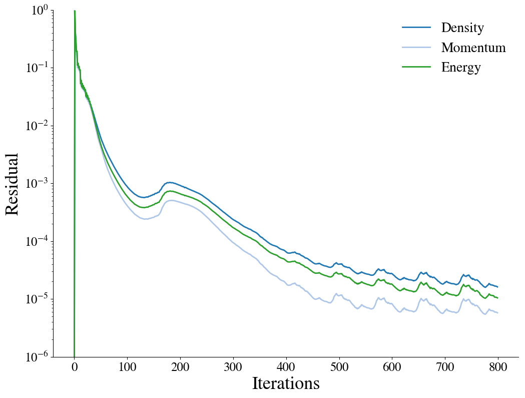
Furthermore, the convergence of the density, momentum and energy equations' residuals are shown as a function of the number of iterations:
from IPython.display import Image, HTML, display
from glob import glob
imagesList=''.join( ["<img style='width: 415px; margin: 10px; float: left; border: 0px solid black;' src='%s' />" % str(s)
                 for s in sorted(glob('screenShot/results/conv*.png')) ])
display(HTML(imagesList))
Results
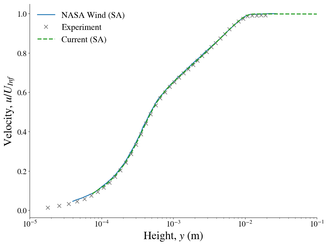
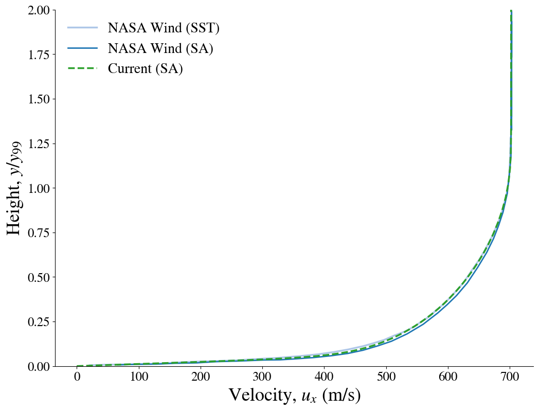
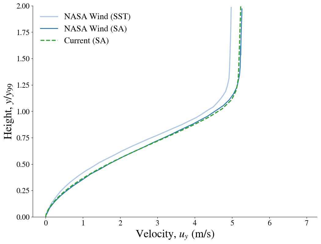
The boundary layer profiles are shown below and compared to the results presented on the NPARC validation website for WIND using the structured mesh. In the upper figure, the streamwise logarithmic profile is compared to experimental measurements.
from IPython.display import Image, HTML, display
from glob import glob
imagesList=''.join( ["<img style='width: 415px; margin: 2px; float: left; border: 0px solid black;' src='%s' />" % str(s)
                 for s in sorted(glob('screenShot/results/U*.png')) ])
display(HTML(imagesList))
from IPython.core.display import HTML

def css_styling():
    styles = open("./styles/custom.css", "r").read()
    return HTML(styles)
css_styling()