import pandas as pd
import numpy as np
import matplotlib as plt
from IPython.display import Image
ONERA M6
This validation case consideres the ONERA M6 wing from the NPARC Alliance Validation and Verification Archive. Below, the results from the high speed aerodynamic solver (HiSA) are compared to the results from WIND and NPARC.
Material properties
It is assumed the fluid can be treated as an ideal gas and the following material properties used:
mP = pd.read_csv('./input/matProp.csv')
mP
Initial conditions
The input parameters, in imperial units, provided in NPARC archive for the freestream conditions are shown below. From the current estimates it appears that these inlet conditions correspond to a Reynolds number of 46x10$^6$ and not the experimental value of 11.72x10$^6$. To recover a Reynolds number of 11.72x10$^6$ a static pressure of 11.677 psia should be specified.
iCI = pd.read_csv('./input/intialCondImp.csv')
iCI
From these input parameters, SI units for HiSA are computed. The freestream or static temperature, $T$, in kelvin is
tempKelvin = iCI.iloc[0][2]*5.0/9.0
print("%.3f K" % tempKelvin)
and the freestream presure, $p_{\infty}$, in Pascals is
pressPascal = iCI.iloc[0][1]*6894.75729
print("%.3f Pa" % pressPascal)
If the acoustic velocity, $c$, is
c = np.sqrt(mP.iloc[0][1]*mP.iloc[0][0]*tempKelvin)
print("%.3f m/s" % c)
then the prescribed inlet velocity vector $u$ is
u = iCI.iloc[0][0]*c
#print u
ux = u*np.cos(iCI.iloc[0][3]*np.pi/180.0)
uy = u*np.sin(iCI.iloc[0][3]*np.pi/180.0)
print("( %.3f %.3f 0.0 ) m/s if AoA = %.2f" % (ux,uy,iCI.iloc[0][3]))
Grid
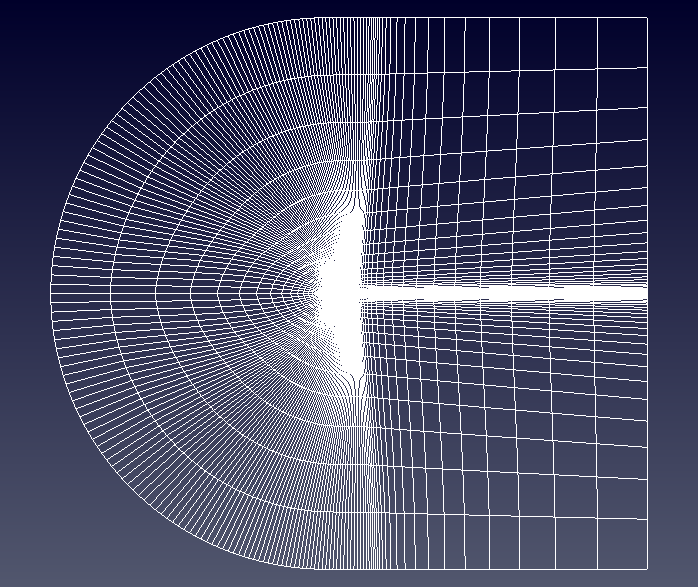
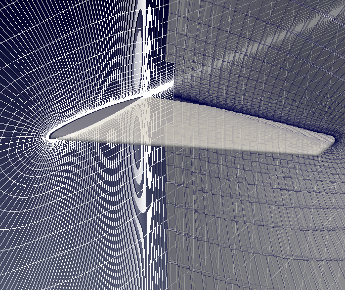
The multiblock, PLOT3D grid from NPARC is imported. It is a C-grid, with 4 zones, wrapping around the leading edge.
| Zone | Dimension | Total Grid Points |
| 1 | 25x49x33 | 40425 |
| 2 | 73x49x33 | 118041 |
| 3 | 73x49x33 | 118041 |
| 4 | 25x49x33 | 40425 |
To construct the Neutral Map File for mesh conversion, it is noted that the JMin surface of zone 2 contains the lower surface of the wing and JMin of zone 3 the upper surface. The JMax surfaces of the all the zones form the farfield boundary. The KMin surfaces coincide with the symmetry plane, whereas the KMax boundaries are coupled as they envelope the wing tip. The IMin surface of zone 1 and IMax of zone 4 are the outlet boundary and the remaining surfaces are coupled, forming internal patches. To resolve the turbulent boundary layer a wall function boundary condition is required as the first grid point is placed 1.524e-5 m from the wall corresponding to a $y^+$ value smaller than 30.
A single block Plot3D grid for the Onera M6 wing is available from the CFL3D Test/Validation archive.
from IPython.display import Image, HTML, display
from glob import glob
imagesList=''.join( ["<img style='width: 600px; margin: 10px; float: left; border: 0px solid black;' src='%s' />" % str(s)
                 for s in sorted(glob('screenShot/mesh/mesh*.png')) ])
display(HTML(imagesList))
Turbulence model
For the analysis the "Standard"-Spalart-Allmaras implementation is prescibed. Using Sutherland's Law $$\mu = \mu_{0} \left( \frac{T}{T_{0}} \right)^{3/2}\frac{T_{0} + S}{T + S}$$ and noting the requirements on the boundary conditions $$\tilde \nu_{wall} = 0 \quad \text{and} \quad \tilde 3 \nu_{\infty} < \nu_{\infty} < 5 \nu_{\infty}$$ the freestream value for $\tilde \nu_{\infty}$ can be calculated
# Sutherland
mu0 = 1.716e-5
T0  = 273.15
S   = 110.4
C1  = 1.458e-6
mu  = mu0*np.power(tempKelvin/T0,1.5)*(T0 + S)/(tempKelvin + S)
# Ideal gas density
rho = pressPascal/(mP.iloc[0][0]*tempKelvin)
# print(rho)
# Kinematic viscosity
nu  = mu/rho
# Freestream nuTilda
nuTilda = 4*nu
print("%.4e m^2/s" % nuTilda)
For the wing the reference length the mean aerodynamic chord is used.
rV = pd.read_csv('./input/refValues.csv')
rV
The corresponding Reynolds number, $\mathrm{Re}$, is
Re = rho*u*rV.iloc[0][0]/mu
print("%.2f" % Re)
To recover a $y^+$ of 1, the wall distance, $y$, should be less than
if (Re > 1e9):
    print ("******************************************************************************")
    print ("WARNING: The Schlichting skin-friction correlation is only valid for Re < 10e9")
    print ("******************************************************************************")
# Schlichting skin-friction correlation
Cf    = np.power(2*np.log10(Re)-0.65,-2.3)
# Wall shear stress
tauW  = 0.5*Cf*rho*u*u
# Friction velocity
uStar = np.sqrt(tauW/rho)
# Wall distance
yPlus = 1
y     = yPlus*mu/(rho*uStar)
print("%.4e m" % y)
and for $y^+$ of 30, the first grid point should be placed at
yPlus = 30
y     = yPlus*mu/(rho*uStar)
print("%.4e m" % y)
Running
A number of scripts are provided to set up the case and run the simulation. To generate the mesh navigate to the case directory, oneraM6, and execute the scripts ./cleanMesh and ./setupMesh. The setupMesh script execute the follow commands
| p2d2p3d | Extrude and convert the 2D PLOT3D mesh to 3D format | |
| p3d2gmsh | Convert the PLOT3D mesh to GMSH | |
| gmshToFoam | Import GMSH into FOAM | |
| stitchMesh | Remove internal patches left over from PLOT3D | |
| changeDictionary | Rename the viscous wall boundary type to 'wall' 1 | |
| 1 Requirement from turbulent model as it searches the 'wall' patches when calculating the near wall distance. | ||
Next, to run the simulation the ./cleanSim and ./runSim scripts should be executed. The runSim script creates a symbolic link to the mesh files in the folder mesh and executes the solver across multiple cores.
Convergence
To examine the solution convergence, first, the engineering quantities are evaluated. Here the lift and drag on the airfoil are plotted against the number of iterations.
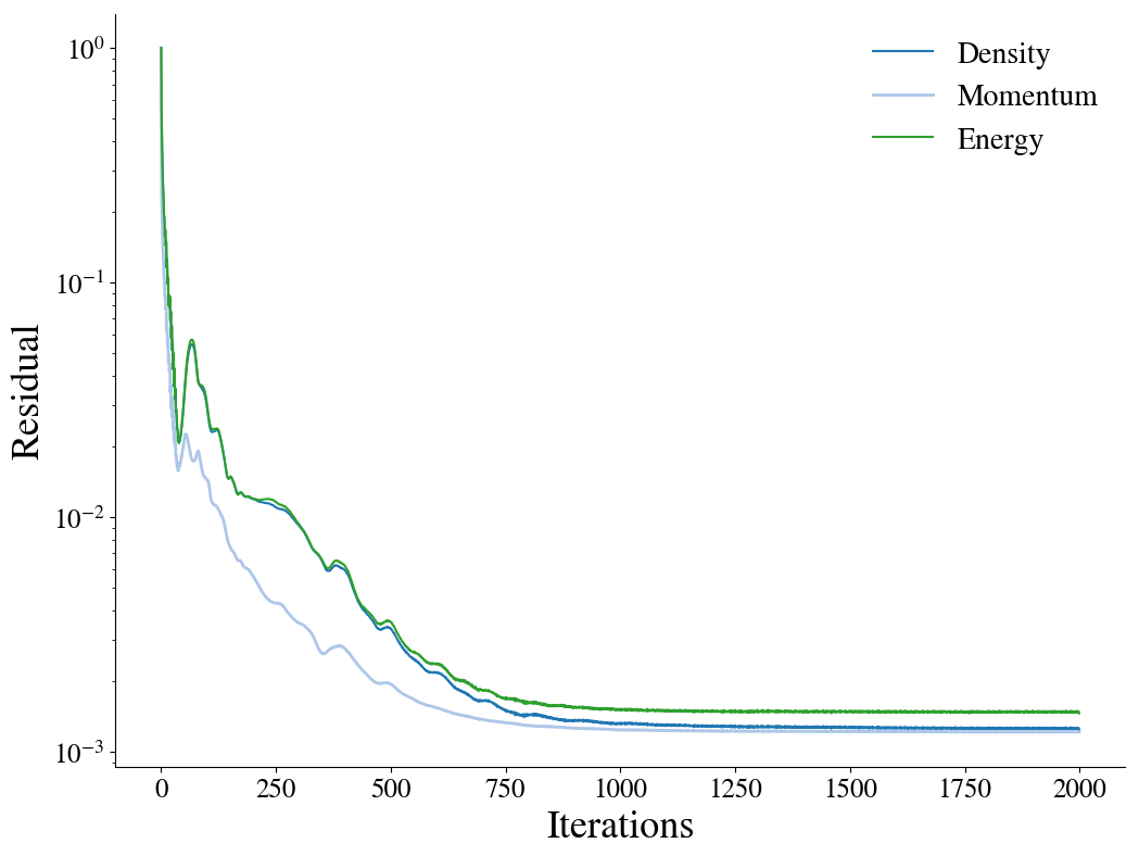
To examine the solution convergence, the density, momentum and energy equations' residuals are shown as a function of the number of iterations:
from IPython.display import Image, HTML, display
from glob import glob
imagesList=''.join( ["<img style='width: 415px; margin: 10px; float: left; border: 0px solid black;' src='%s' />" % str(s)
                 for s in sorted(glob('screenShot/results/conv*.png')) ])
display(HTML(imagesList))
Results
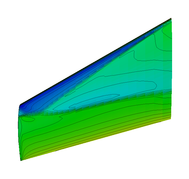
The pressure contour plots of the upper surface are shown for CFL3D, on the left, and HiSA, on the right. The CFL3D results are taken from the CFL3D Test/Validation archive.
from IPython.display import Image, HTML, display
from glob import glob
imagesList=''.join( ["<img style='width: 310px; margin: 10px; float: left; border: 0px solid black;' src='%s' />" % str(s)
                 for s in sorted(glob('screenShot/results/pressCont*.png')) ])
display(HTML(imagesList))

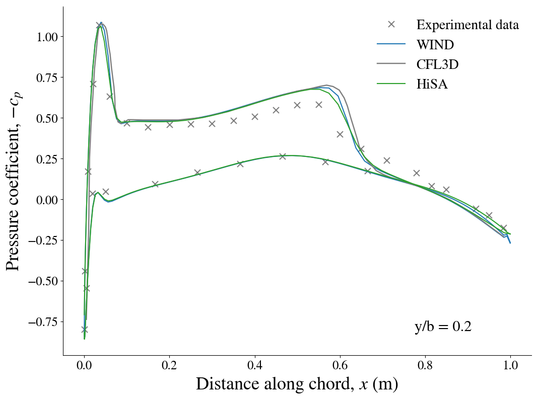
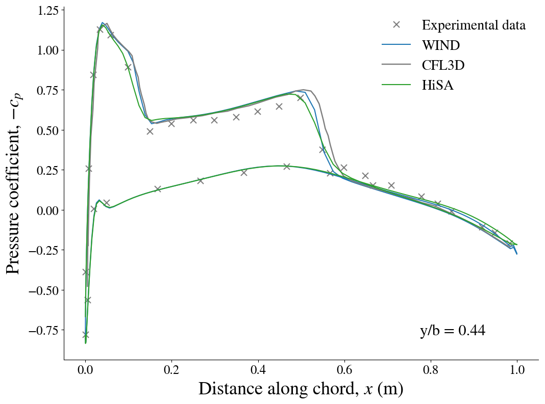
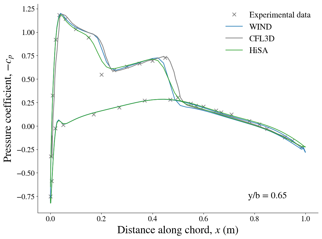
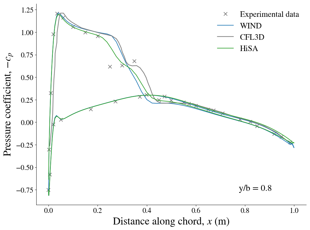
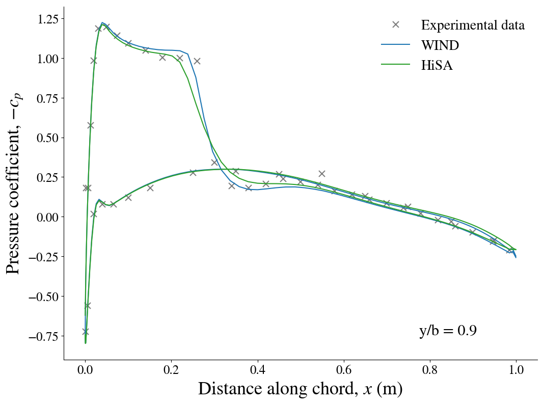
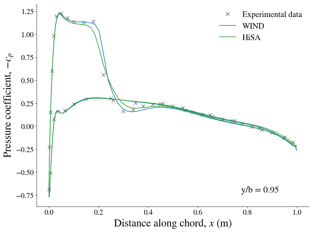
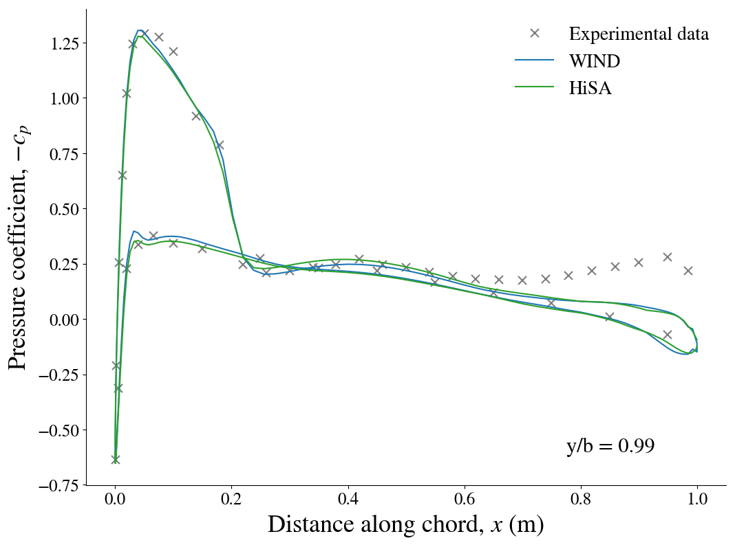
Below, the cross-sectional pressure coefficients at various sections of the wing are shown. The experimental results are shown along with the numerical predictions from WIND, CFL3D as well as HiSA. The WIND and HiSA results are obtained using the Spalart-Allmaras turbulence model with wall functions.
from IPython.display import Image, HTML, display
from glob import glob
imagesList=''.join( ["<img style='width: 415px; margin: 10px; float: left; border: 0px solid black;' src='%s' />" % str(s)
                 for s in sorted(glob('screenShot/results/cp*.png')) ])
display(HTML(imagesList))
from IPython.core.display import HTML

def css_styling():
    styles = open("./styles/custom.css", "r").read()
    return HTML(styles)
css_styling()