In [1]:

import pandas as pd
import numpy as np
import matplotlib as plt
from IPython.display import Image

RAE Transonic Airfoil¶

This validation case consideres the RAE Transonic Airfoil from the NPARC Alliance Validation and Verification Archive, in particular Study 4. Below the results from the high speed aerodynamic solver (HiSA) are compared to the results from WIND and NPARC.

Material properties¶

It is assumemd the fluid can be treated as an ideal gas and the following material properties used:

In [2]:

mP = pd.read_csv('./input/matProp.csv')
mP

Out[2]:

	Gas constant	Specific heat ratio
0	287.058	1.4

Initial conditions¶

The NPARC archive provides the following input parameters, in imperial units, for the freestream conditions:

In [3]:

iCI = pd.read_csv('./input/intialCondImp.csv')
iCI

Out[3]:

	Mach Number	Static Pressure	Temperature	Angle-of-Attack
0	0.729	15.80734	460.0	2.31

From these input parameters, SI units for HiSA are computed. The freestream or static temperature, $T$, in kelvin is

In [4]:

tempKelvin = iCI.iloc[0][2]*5.0/9.0
print("%.3f K" % tempKelvin)

255.556 K

and the freestream pressure, $p_{\infty}$, in Pascals is

In [5]:

pressPascal = iCI.iloc[0][1]*6894.75729
print("%.3f Pa" % pressPascal)

108987.773 Pa

If the acoustic velocity, $c$, is

In [6]:

c = np.sqrt(mP.iloc[0][1]*mP.iloc[0][0]*tempKelvin)
print("%.3f m/s" % c)

320.473 m/s

then the prescribed inlet velocity vector $u$ is

In [7]:

u = iCI.iloc[0][0]*c
ux = u*np.cos(iCI.iloc[0][3]*np.pi/180.0)
uy = u*np.sin(iCI.iloc[0][3]*np.pi/180.0)
print("( %.3f 0.0 %.3f ) m/s if AoA = %.2f" % (ux,uy,iCI.iloc[0][3]))

( 233.435 0.0 9.417 ) m/s if AoA = 2.31

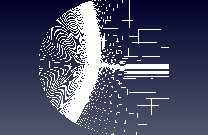
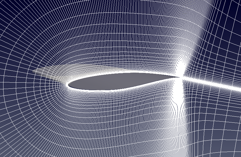
Grid¶

The PLOT3D grid from NPARC is imported. It is a single-block, two-dimensional C-grid with dimensions of 369 x 65. To construct the Neutral Map File for mesh conversion, it is noted that airfoil surface and wake are located at the JMin boundary. The I-coordinate starts at the lower outflow boundary, runs around the airfoil and continues back to the outflow boundary. It intersects the airfoil's trailing edge at I33, proceeds along the bottom of the airfoil, around the leading edge, downstream along the top of the airfoil and intersects the trailing edge again at I337.

In [8]:

from IPython.display import Image, HTML, display
from glob import glob
imagesList=''.join( ["<img style='width: 550px; margin: 10px; float: left; border: 0px solid black;' src='%s' />" % str(s) 
                 for s in sorted(glob('screenShot/mesh/mesh*.png')) ])
display(HTML(imagesList))

Turbulence model¶

For the analysis the "Standard"-Spalart-Allmaras implementation is prescibed. Using Sutherland's Law $$\mu = \mu_{0} \left( \frac{T}{T_{0}} \right)^{3/2}\frac{T_{0} + S}{T + S}$$ and noting the requirements on the boundary conditions $$\tilde \nu_{wall} = 0 \quad \text{and} \quad 3 \nu_{\infty} < \tilde \nu_{\infty} < 5 \nu_{\infty}$$ the freestream value for $\tilde \nu_{\infty}$ can be calculated

In [9]:

# Sutherland
mu0 = 1.716e-5
T0  = 273.15
S   = 110.4
C1  = 1.458e-6
mu  = mu0*np.power(tempKelvin/T0,1.5)*(T0 + S)/(tempKelvin + S)
# Ideal gas density
rho = pressPascal/(mP.iloc[0][0]*tempKelvin)
#print(rho)
# Kinematic viscosity
nu  = mu/rho
# Freestream nuTilda
nuTilda = 4*nu
print("%.4e m^2/s" % nuTilda)

4.3820e-05 m^2/s

For the airfoil the reference length is taken to be the chord length and the reference area is the product of the actual airfoil width and the chord length. The centre of rotation is 0.25 % from the leading edge.

In [10]:

rV = pd.read_csv('./input/refValues.csv')
rV

Out[10]:

	Length	Area	Centre of rotation
0	0.3048	0.3048	0.07585

The corresponding Reynolds number, $\mathrm{Re}$, is

In [11]:

Re = rho*u*rV.iloc[0][0]/mu
print("%.2f" % Re)

6500094.74

To recover a $y^+$ of 1, the wall distance, $y$, should be less than

In [12]:

if (Re > 1e9):
    print ("******************************************************************************")
    print ("WARNING: The Schlichting skin-friction correlation is only valid for Re < 10e9")
    print ("******************************************************************************")
# Schlichting skin-friction correlation
Cf    = np.power(2*np.log10(Re)-0.65,-2.3)
# Wall shear stress
tauW  = 0.5*Cf*rho*u*u
# Friction velocity
uStar = np.sqrt(tauW/rho)
# Wall distance
yPlus = 1
y     = yPlus*mu/(rho*uStar) 
print("%.4e m" % y)

1.2639e-06 m

and for $y^+ < 30$, $y$ should be smaller than

In [13]:

yPlus = 30
y     = yPlus*mu/(rho*uStar) 
print("%.4e m" % y)

3.7917e-05 m

Running¶

A number of scripts are provided to set up the case and run the simulation. To generate the mesh navigate to the case directory, rae2822, and execute the scripts ./cleanMesh and ./setupMesh. The setupMesh script executes the follow commands

p2d2p3d	Extrude and convert the 2D PLOT3D mesh to 3D format
p3d2gmsh	Convert the PLOT3D mesh to GMSH
gmshToFoam	Import GMSH into FOAM
stitchMesh	Remove internal patches left over from PLOT3D
changeDictionary	Rename the viscous wall boundary type to 'wall' ¹
¹ Requirement from turbulent model as it searches the 'wall' patches when calculating the near wall distance.

Next, to run the simulation the ./cleanSim and ./runSim scripts should be executed. The runSim script create a symbolic link to the mesh files in the folder mesh and execute the solver across multiple cores.

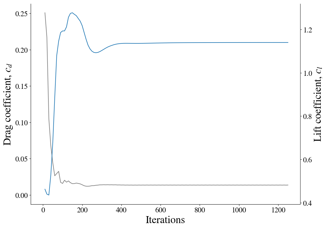
Convergence¶

To examine the solution convergence, first, the engineering quantities are evaluated. Here the lift and drag on the airfoil are plotted against the number of iterations.

In [14]:

from IPython.display import Image, HTML, display
from glob import glob
imagesList=''.join( ["<img style='width: 415px; margin: 10px; float: left; border: 0px solid black;' src='%s' />" % str(s) 
                 for s in sorted(glob('screenShot/results/*Conv.png')) ])
display(HTML(imagesList))

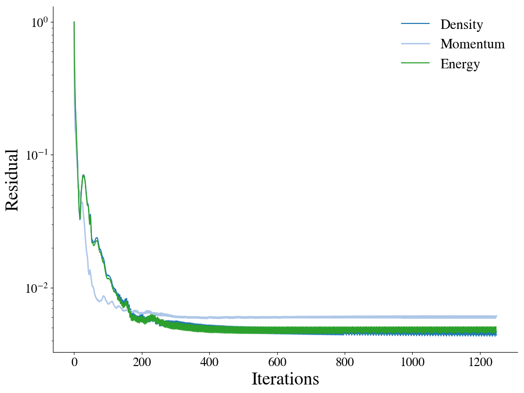
Furthermore, the convergence of the density, momentum and energy equations' residuals are shown as a function of the number of iterations:

In [15]:

from IPython.display import Image, HTML, display
from glob import glob
imagesList=''.join( ["<img style='width: 415px; margin: 10px; float: left; border: 0px solid black;' src='%s' />" % str(s) 
                 for s in sorted(glob('screenShot/results/conv*.png')) ])
display(HTML(imagesList))

Results¶

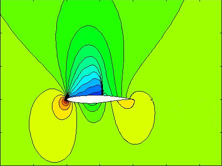
The pressure contour plot for HiSA is shown along side the results presented on the NPARC validation website.

In [16]:

from IPython.display import Image, HTML, display
from glob import glob
imagesList=''.join( ["<img style='width: 310px; margin: 10px; float: left; border: 0px solid black;' src='%s' />" % str(s) 
                 for s in sorted(glob('screenShot/results/pressCont*.png')) ])
display(HTML(imagesList))

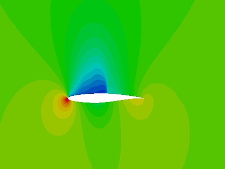
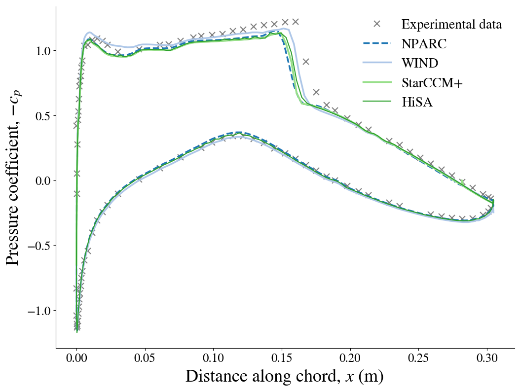
The figure below presents a comparison between the numerical results from HiSA, the predictions from NPARC and WIND as well as experimental data. The WIND results are obtained from a Spalart-Allmaras turbulence analysis.

In [17]:

from IPython.display import Image, HTML, display
from glob import glob
imagesList=''.join( ["<img style='width: 415px; margin: 10px; float: left; border: 0px solid black;' src='%s' />" % str(s) 
                 for s in sorted(glob('screenShot/results/cp.png')) ])
display(HTML(imagesList))

In [18]:

from IPython.core.display import HTML

def css_styling():
    styles = open("./styles/custom.css", "r").read()
    return HTML(styles)
css_styling()

Out[18]: